Quickstart

Let’s build a closed loop on the canvas: a setpoint, a PID controller and a plant. You will run it, plot it and tune it, then find out that you were writing a text file all along.

Create a project

Install magnet first if you haven’t. Then:

magnet new hello && cd hello
magnet gui

magnet new scaffolds the project and makes it a git repository (--no-git skips that). magnet gui opens the editor in your browser.

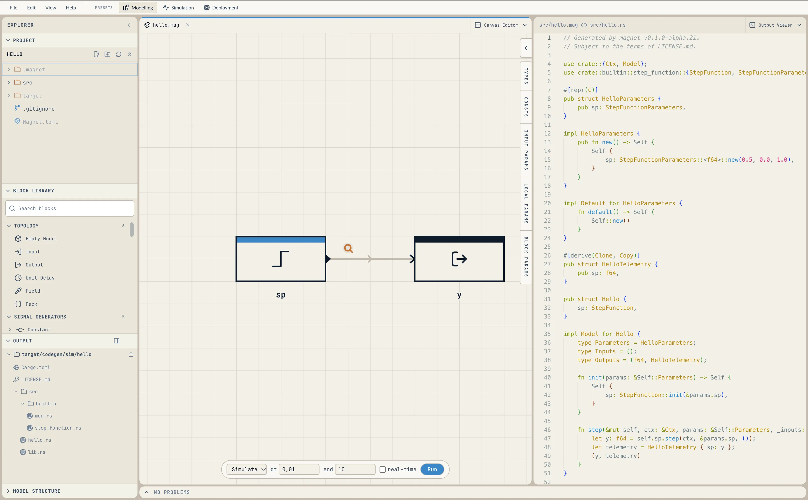
The starter model is a step source sp wired to an output y. The step jumps from 0 to 1 at t = 0.5, and it will be the setpoint of the loop.

Build the loop

Hover over the canvas and press Shift + A to open the block picker. Type a block’s name and press Enter to place it under the cursor. You can also drag blocks from the Block Library on the left.

Place three blocks:

• Control Sum, to compare the setpoint with the measurement. It subtracts its second input from its first, so its output is the error.
• PID, the controller.
• Integrator, the plant. Think of it as a tank you fill: the controller sets the flow, and the level is what you measure.

Wire them by dragging from an output port to an input port:

1. sp to the Control Sum’s first input.
2. Control Sum to PID.
3. PID to Integrator.
4. Integrator to y. A wire dropped on a connected input replaces the old one.
5. Integrator back to the Control Sum’s second input, to close the loop.

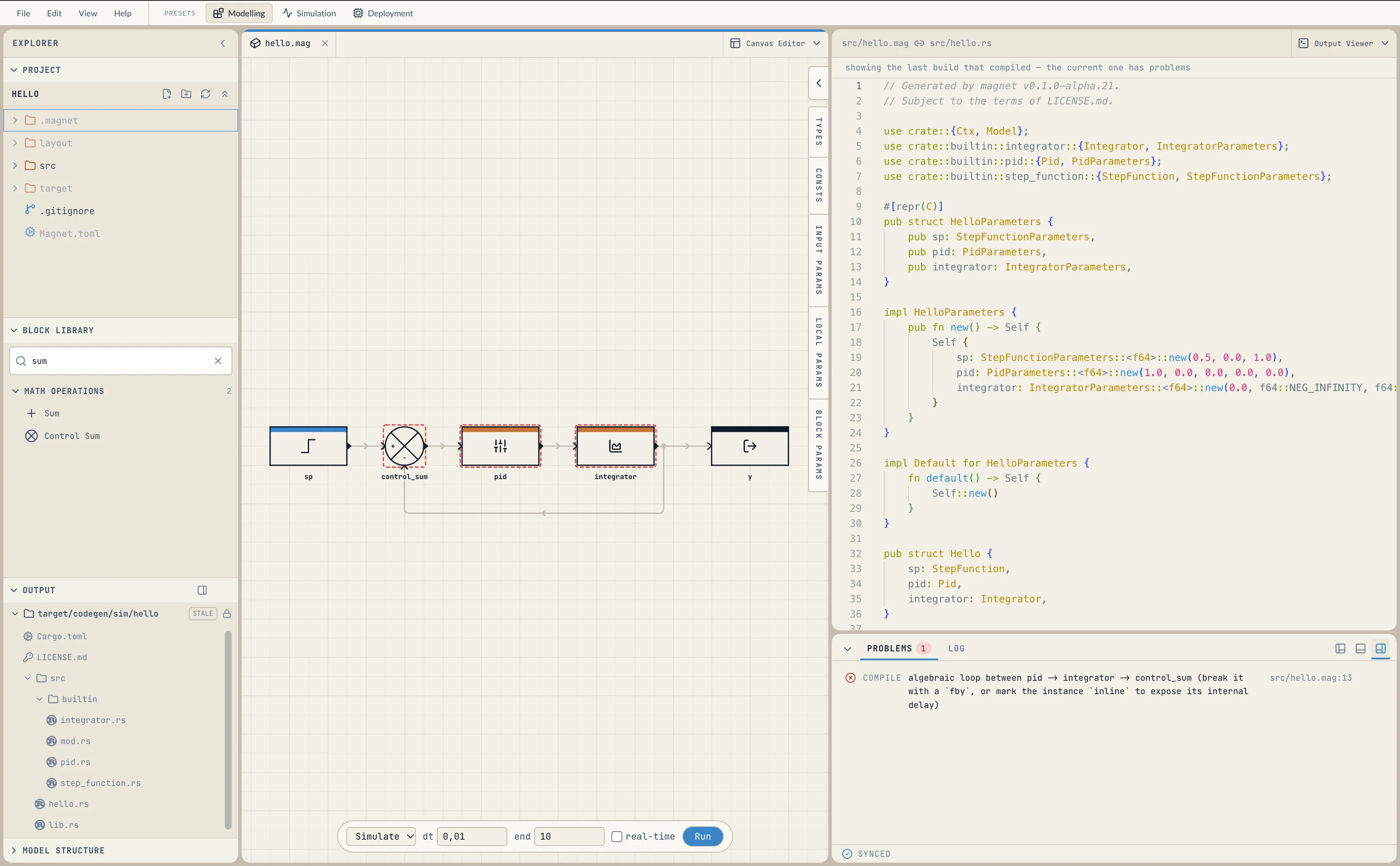
The loop turns red, and the Problems panel reports an algebraic loop. Each block’s output depends on its input in the same tick, so the cycle has no valid order, and Magnetite refuses to guess one.

Break the algebraic loop

Place a Unit Delay below the loop. Wire the Integrator to it, and wire its output to the Control Sum’s second input. The Control Sum now compares against the measurement from one tick ago, and the problem clears.

Causality, delays and feedback explains why the delay is needed and the other ways to break a loop.

Probe and run

The starter model already probes sp. Hover over the Integrator’s output wire and click the probe icon to probe it too. Probed signals are recorded on every run.

Press Run at the bottom of the canvas. The first run compiles the generated Rust, which takes a moment, and later runs reuse that build.

Switch to the Simulation preset on the top bar to see the results. Probes plots each probed signal on its own. To overlay them, open Custom Plots, press Add plot, choose Hello::sp and Hello::integrator, and press Apply.

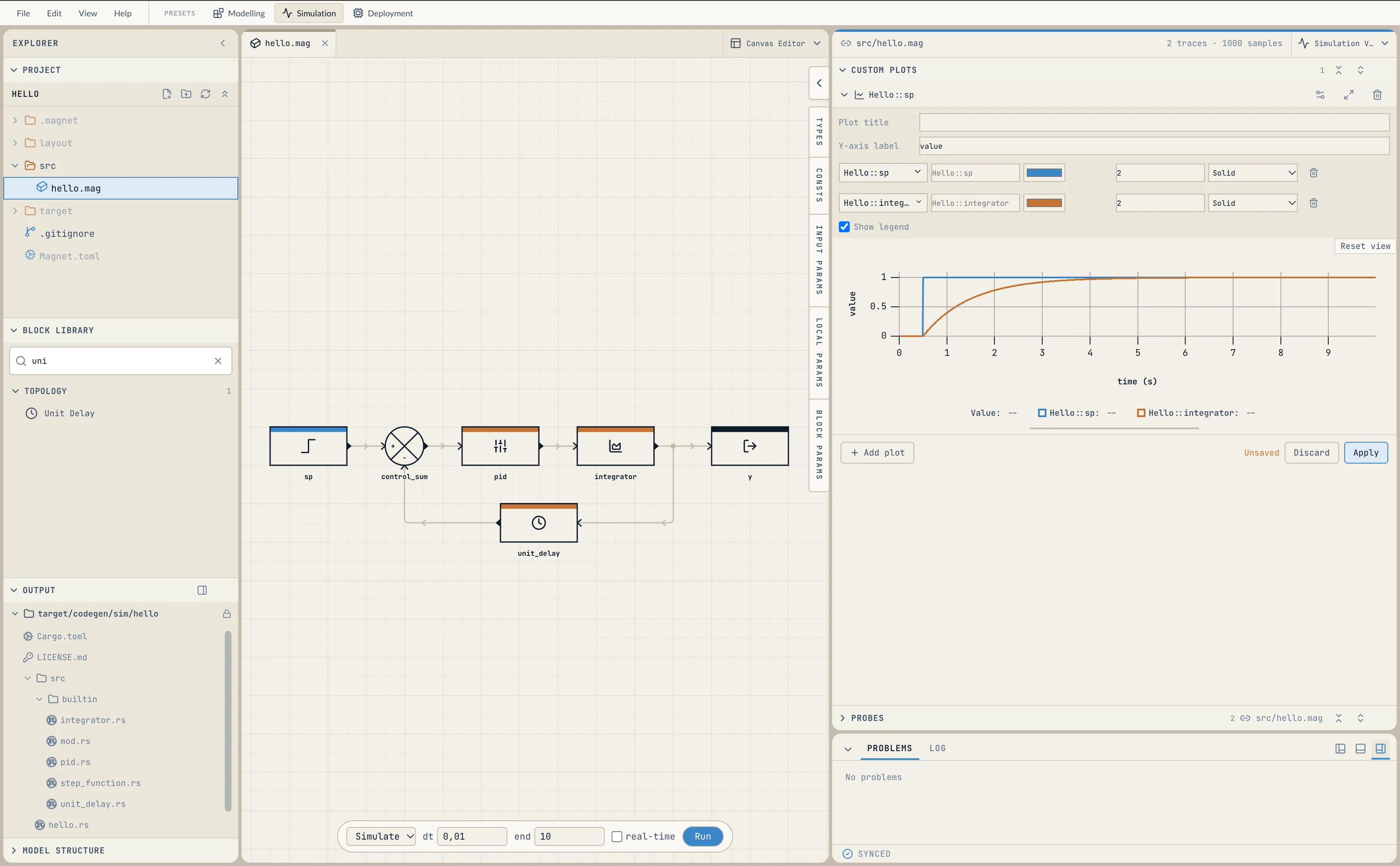
The plant output rises to meet the setpoint, but it takes about four seconds.

Tune it

Double-click the PID block. The gains start at Kp = 1, Ki = 0 and Kd = 0. Set Kp to 4.0, press Apply, and run again.

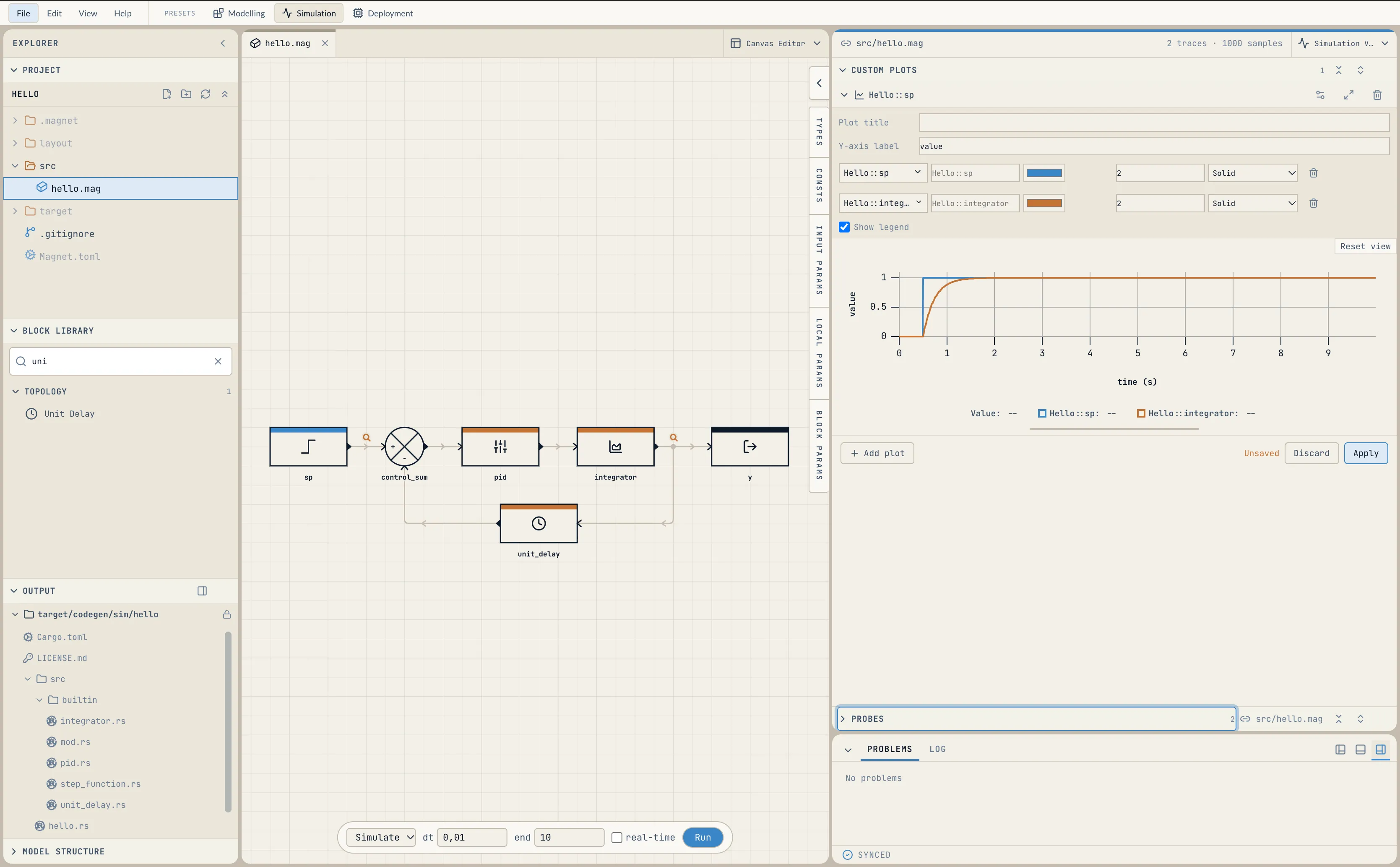
The response is now about four times faster. Try Ki and Kd as well, and run after each change: place, wire, run, read and adjust is the loop you will work in.

Read the text

Everything you did on the canvas was written to src/hello.mag. To see it beside the diagram, right-click hello.mag in the explorer and choose Open in Text Editor.

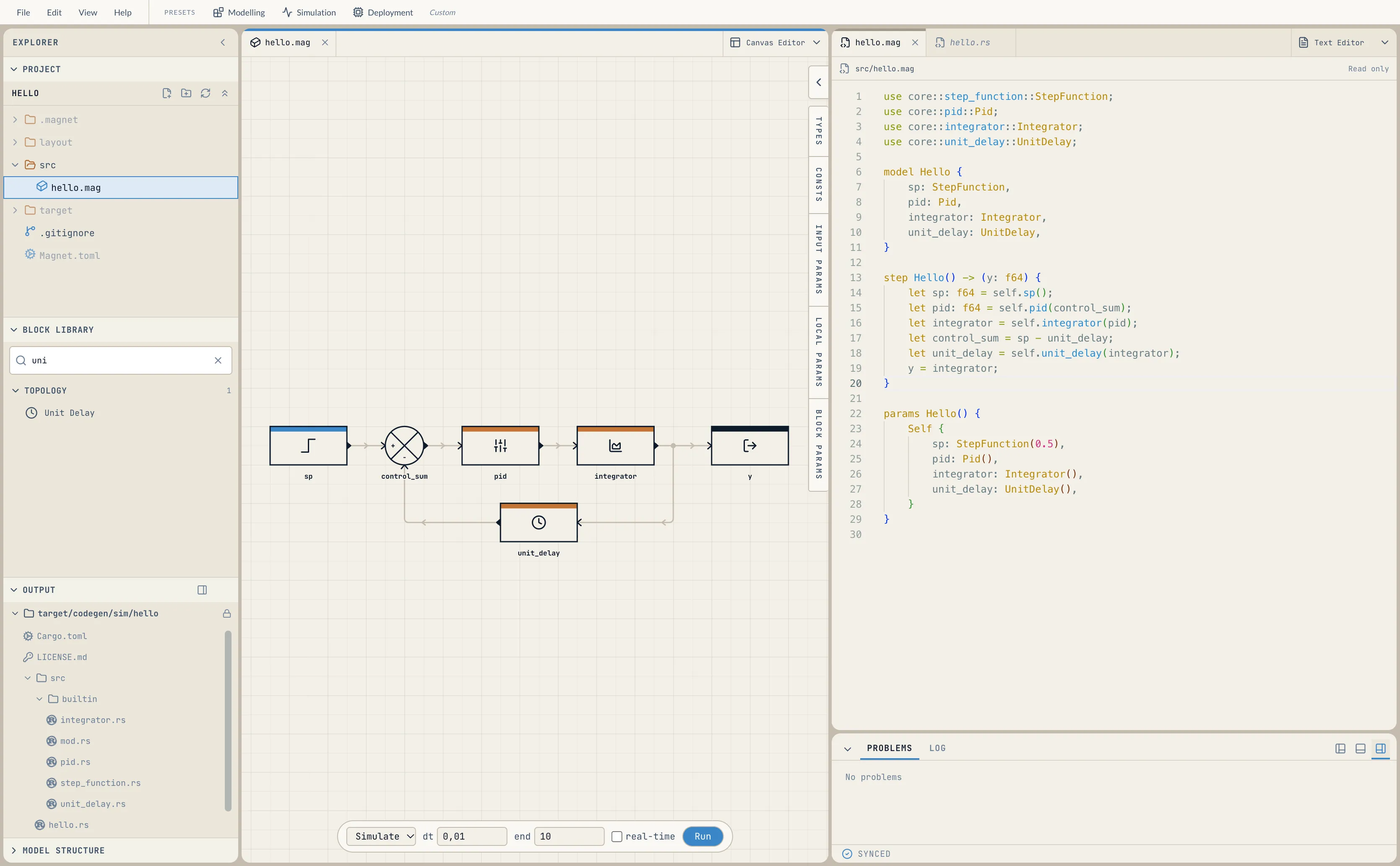
After tuning, the file reads:

use core::step_function::StepFunction;
use core::pid::Pid;
use core::integrator::Integrator;
use core::unit_delay::UnitDelay;

model Hello {
    sp: StepFunction,
    pid: Pid,
    integrator: Integrator,
    unit_delay: UnitDelay,
}

@probe(sp, integrator)
step Hello() -> (y: f64) {
    let sp: f64 = self.sp();
    let pid: f64 = self.pid(control_sum);
    let integrator = self.integrator(pid);
    let control_sum = sp - unit_delay;
    let unit_delay = self.unit_delay(integrator);
    y = integrator;
}

params Hello() {
    Self {
        sp: StepFunction(0.5),
        pid: Pid(4.0),
        integrator: Integrator(),
        unit_delay: UnitDelay(),
    }
}

These four constructs are the whole shape of a Magnetite file:

1. model declares the blocks that keep state between ticks, one field each.
2. step is the per-tick function: typed inputs and outputs, and a body of equations. Every output is assigned exactly once.
3. @probe(...) marks signals for telemetry. Each one becomes a trace.
4. params builds the model. StepFunction(0.5) sets the step time and Pid(4.0) sets Kp. Arguments left out take their defaults.

The Control Sum has no field because it keeps no state: it is the expression sp - unit_delay. The equations in a step hold simultaneously, so control_sum and unit_delay can be read before the lines that define them.

The canvas and the text are one model. The editor’s text pane is read-only, but you can edit the file in your own editor, and the canvas follows when you save.

Run it from the command line

The same project runs without the editor. Without a path argument, a command acts on the project around the working directory, found by walking up to Magnet.toml.

$ magnet check
    Checking hello
          ok 1 model (Hello), 0 functions
$ magnet simulate --dt 0.1 --ticks 10
    Checking hello
    Finished `release` profile [optimized] target(s) in 0.01s
     Running 10 ticks
tick,t,y,probe.sp,probe.integrator
0,0,0,0,0
1,0.1,0,0,0
2,0.2,0,0,0
3,0.30000000000000004,0,0,0
4,0.4,0,0,0
5,0.5,0,1,0
6,0.6000000000000001,0.4,1,0.4
7,0.7000000000000001,0.8,1,0.8
8,0.8,1.04,1,1.04
9,0.9,1.12,1,1.12

The CSV has a tick counter, the simulated time t, one column per output, and one probe. column per probe. At this coarse time step the plant overshoots the setpoint a little.

Progress lines go to stderr, so magnet simulate > out.csv writes only CSV. The CLI reference covers the rest, including --param for overriding a parameter for one run.

What is in the project

Path	Holds	Commit it?
Magnet.toml	The manifest: the package name and its dependencies	Yes
src/	The .mag files, each one a module	Yes
layout/	Where the blocks sit on the canvas, one file per .mag	Yes
.magnet/	Derived state the editor and CLI keep while working	No
target/codegen/	The generated Rust crates and their build output	No

.magnet/ and target/ are gitignored and fully derived, so deleting either is safe.

Next

• A simple motor and controller writes a model with real inputs in text.
• Satellite attitude control builds a complete controller.
• Modules explains how files, models and use paths fit together.